Circuit Solver and Simulator: A Deep Dive into Electrical Networks 🙂✨

This document details the development of my circuit solver and simulator capable of analyzing and visualizing the behavior of electrical circuits. The project goes beyond the introductory circuit analysis covered in class by exploring advanced techniques such as nodal analysis and incorporating interactive visualization. This report documents the theoretical components, implementation details, and practical applications of the developed software, hopefully allowing readers to gain a more comprehensive understanding of electrical circuit principles than they started with.

1. Introduction

Understanding electrical circuits is fundamental to modern technology. While basic circuit analysis techniques like series and parallel resistor combinations provide a foundation, real-world circuits often require more sophisticated methods. This project aims to bridge the gap between theoretical concepts and practical application by creating a software tool that can:

Solve for node voltages and branch currents in complex circuits using nodal analysis.
Simulate the dynamic behavior of circuits containing capacitors and inductors.
Provide a user-friendly interface for circuit design and visualization

This project not only reinforces the concepts learned in class but also expands upon them by exploring numerical methods for solving complex circuit configurations and providing a foundation for future development of interactive graphical representations of circuit behavior.

2. Theoretical Background

2.1 Nodal Analysis

Nodal analysis is a very powerful technique for solving complex circuits. It's based on Kirchhoff's Current Law (which simply states that the algebraic sum of currents entering a node is zero). By applying KCL at each non-reference node in a circuit, you can obtain a system of linear equations that can be solved to find the node voltages. These voltages can then be used to determine branch currents using Ohm's Law.

For a node $i$ with voltage $V_i$ , connected to nodes $j$ with conductance $G_{ij}$ , and with independent current sources $I_i$ entering the node, KCL gives:

$\sum_{j \ne i} G_{ij}(V_i - V_j) = I_i$

This can be rearranged into a matrix equation of the form:

$\mathbf{V} \mathbf{G} = \mathbf{I}$

where $\mathbf{G}$ is the conductance matrix, $\mathbf{V}$ is the vector of node voltages, and $\mathbf{I}$ is the vector of independent current sources. Solving for $\mathbf{V}$ involves matrix inversion or other numerical methods.

Matrix inversion is the process of finding a matrix that, when multiplied by the original matrix, results in the identity matrix. The identity matrix is just the original matrix but with $1$ 's along its main diagonal (from the top-left to the bottom-right) and zeros elsewhere:

$I_2 = \begin{bmatrix} 1 & 0 \\ 0 & 1 \end{bmatrix}\quad\quad I_3 = \begin{bmatrix} 1 & 0 & 0 \\ 0 & 1 & 0 \\ 0 & 0 & 1 \end{bmatrix}$

While important, a deep dive into the specifics of matrix inversion is outside the scope and focus of my report. So, we'll leave it at that and just take note of the practical usage of the method.

2.2 Circuit Simulation:

For circuits containing capacitors and inductors, the behavior is time-dependent. The governing equations become differential equations:

$\text{Capacitor:} \quad i_C(t) = C \frac{dv_C(t)}{dt}$

$\text{Inductor:} \quad v_L(t) = L \frac{di_L(t)}{dt}$

To simulate these circuits, numerical integration techniques such as the Euler method or more advanced methods like the Runge-Kutta methods are employed to approximate the solutions to these differential equations over time.

Although the implementation of these numerical integration techniques proved to be beyond the scope of this current project iteration due to time constraints, I will still present the detailed mathematical framework and planned code implementation strategy for dynamic circuit simulation, as this remains a key area for future development.

This detailed plan will serve as a valuable personal reference for future development (I will definitely be revisiting this project once I have more time lol...) and as a guide for others who might be interested in extending or utilizing its capabilities. Most of the difficulties I faced throughout this project stemmed from the lack of online resources regarding the simulation implementation and other technical aspects. I hope that anyone in the future attempting to build something similar can learn from my experience.

3. Implementation

The circuit solver and simulator was initially intended to utilize JavaScript (TypeScript) for the user interface and Rust (WASM) for solving equations and performing simulations. However, due to time constraints, the current implementation relies solely on JavaScript. Future development will explore integrating Rust as planned to leverage its performance benefits for the computationally intensive simulation tasks.

3.1 Circuit Representation

The circuit is represented internally as a graph data structure. Nodes represent connection points, and edges represent circuit components (resistors, capacitors, inductors, voltage sources, current sources, etc.). Each component is characterized by its parameters (resistance, capacitance, inductance, voltage, current).

3.1.1 UI to Graph Conversion (Challenges)

A significant challenge in the implementation is translating the user's circuit design from the visual user interface into the underlying graph representation. This involves:

Component Identification and Parameter Extraction: Accurately identifying each UI component (resistors, capacitors, etc.) and extracting relevant parameters (resistance value, orientation, connections) from the UI elements. This requires careful planning for anything related to user interactions and UI events.
Node Mapping: Establishing a consistent mapping between visual connection points in the UI and the nodes in the graph data structure. This is needed for correctly representing circuit topology.
Handling Complex Connections: Addressing scenarios involving complex component interconnections and ensuring the graph accurately reflected these connections. This includes handling potential ambiguities in user-drawn connections.
Invalid Circuit Detection: Implementing robust error handling to detect and report invalid circuit configurations, such as:
- Short Circuits: Identifying direct connections between voltage sources.
- Open Circuits: Handling incomplete circuits or components not connected to the rest of the circuit.
- Invalid Component Configurations: Recognizing and flagging components with incorrect or missing parameters.
- Floating Nodes: Identifying nodes that are not connected to any other part of the circuit (except ground probably...).

3.2 Nodal Analysis Solver

The nodal analysis solver implements the following steps:

Identify Nodes: The algorithm identifies all nodes in the circuit and selects a reference node (ground).
Formulate Conduhctance Matwrix 🤓: The conductance matrix $\mathbf{G}$ is constructed based on the connections and component values between nodes.
Formulate Current Source Vector: The current source vector $\mathbf{I}$ is created based on the independent current sources connected to each nod.
Solve for Node Voltages: The matrix equation $\mathbf{G} \mathbf{V} = \mathbf{I}$ is solved using a linear equation solver (Gaussian elimination) to obtain the node voltage vector $\mathbf{V}$ .
Calculate Branch Currents: Once node voltages are known, then the branch currents are calculated using Ohm's Law and the component values.

3.3 Circuit Simulation Engine

The simulation engine would use a time-stepping approach to solve the differential equations governing the behavior of capacitors and inductors.

Discretize Time: In English, this means time is divided into small discrete steps.
Apply Numerical Integration: At each time step, the voltages and currents of capacitors and inductors are updated using a numerical integration method (Euler method probably):
- Capacitor: $v_C(t + \Delta t) = v_C(t) + \frac{\Delta t}{C} i_C(t)$
- Inductor: $i_L(t + \Delta t) = i_L(t) + \frac{\Delta t}{L} v_L(t)$
Solve for Node Voltages and Branch Currents: At each time step, nodal analysis is performed to determine the node voltages and branch currents, taking into account the updated capacitor and inductor values.
Repeat: Steps 2 and 3 are repeated for each time step to simulate the circuit's behavior over time.

3.4 User Interface:

The user interface (UI) allows users to:

Create Circuits: Drag and drop components (resistors, capacitors, inductors, voltage sources, current sources) onto a canvas to create a circuit diagram.
Edit Component Values: Modify the parameters of each component (resistance, capacitance, inductance, voltage, current).
Run Simulation: Initiate the circuit solver (would have been simulator).
Visualize Results: Display node voltages, branch currents, and waveforms (for time-dependent simulations) graphically.

Editor:

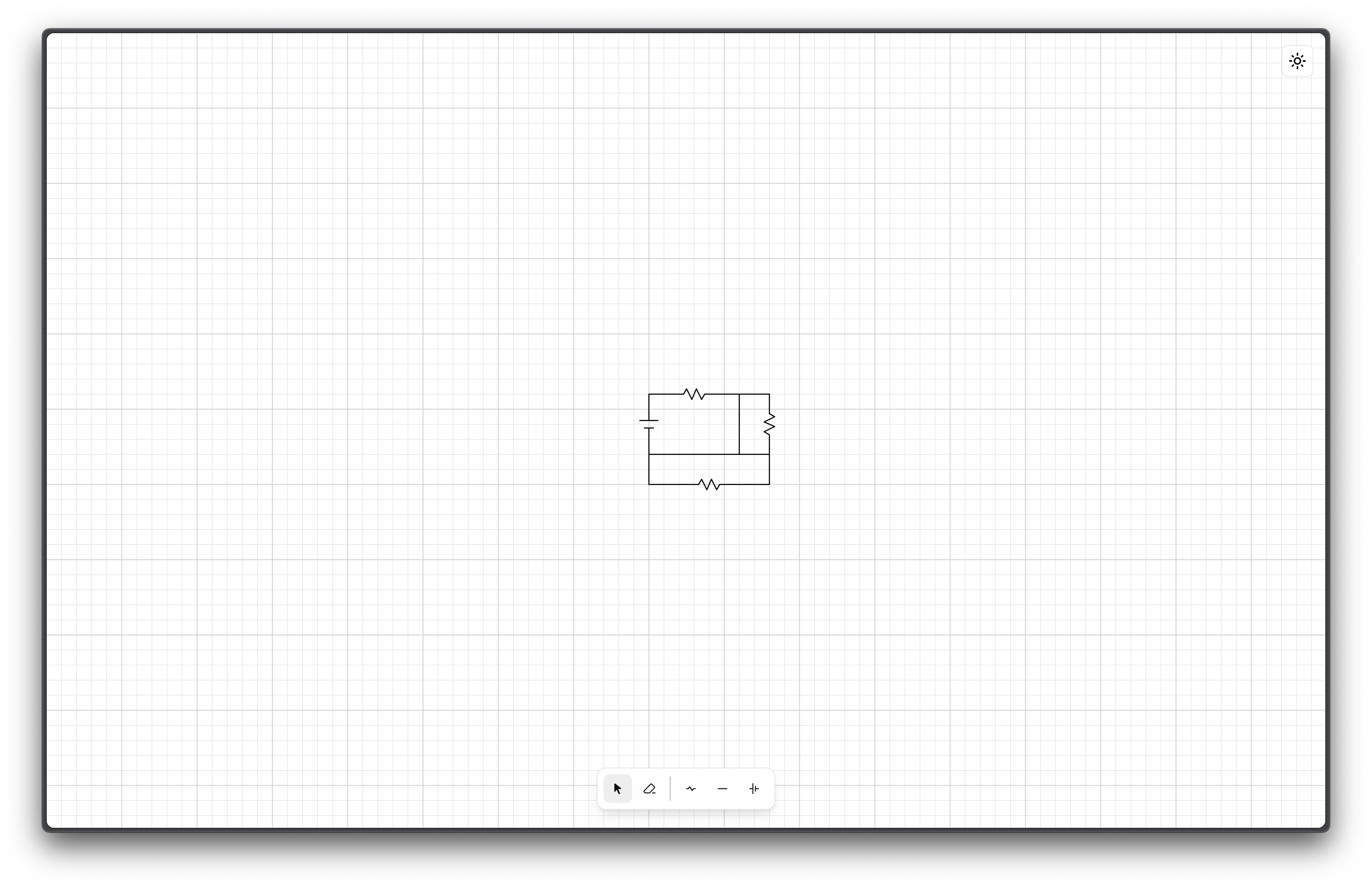
A screenshot of the circuit editor user interface.

4. Quantitative Analysis and Results

// Simplified Example Code For Nodal Analysis Solver (Standalone!!)
const circuit = {
    components: [
        { name: 'V1', type: 'voltageSource', value: 5, nodes: ['V_A', 'GND'] },
        { name: 'R1', type: 'resistor', value: 2, nodes: ['V_A', 'V_B'] },
        { name: 'R2', type: 'resistor', value: 3, nodes: ['V_B', 'GND'] },
        { name: 'R3', type: 'resistor', value: 6, nodes: ['V_B', 'GND'] },
    ],
    nodes: 3,
    nodeNames: ['V_A', 'V_B', 'GND'],
};

const numNodes = circuit.nodes - 1;
let conductanceMatrix = math.zeros(numNodes, numNodes);
let currentMatrix = math.zeros(numNodes, 1);

for (let i = 0; i < numNodes; i++) {
    for (let j = 0; j < numNodes; j++) {
        if (i === j) {
            if (i === 0) {
                conductanceMatrix = math.subset(
                    conductanceMatrix,
                    math.index(i, j),
                    1 / circuit.components[1].value + 1 / circuit.components[2].value
                );
            } else if (i === 1) {
                conductanceMatrix = math.subset(
                    conductanceMatrix,
                    math.index(i, j),
                    1 / circuit.components[2].value + 1 / circuit.components[3].value
                );
            }
        } else {
            if ((i === 0 && j === 1) || (i === 1 && j === 0)) {
                conductanceMatrix = math.subset(
                    conductanceMatrix,
                    math.index(i, j),
                    -1 / circuit.components[2].value
                );
            }
        }
    }
}

currentMatrix = math.subset(
    currentMatrix,
    math.index(0, 0),
    circuit.components[0].value / circuit.components[1].value
);

const voltageMatrix = math.multiply(math.inv(conductanceMatrix), currentMatrix);

const V_A = voltageMatrix.subset(math.index(circuit.nodeNames.indexOf('V_A'), 0));
const V_B = voltageMatrix.subset(math.index(circuit.nodeNames.indexOf('V_B'), 0));

const V_R1 = circuit.components[0].value - V_A;
const V_R2 = V_A - V_B;
const V_R3 = V_B;

console.log('| Component | Value | Calculated Voltage |');
console.log('|---|---|---|');
console.log(`| ${circuit.components[1].name} | ${circuit.components[1].value}Ω | ${V_R1.toFixed(2)}V |`);
console.log(`| ${circuit.components[2].name} | ${circuit.components[2].value}Ω | ${V_R2.toFixed(2)}V |`);
console.log(`| ${circuit.components[3].name} | ${circuit.components[3].value}Ω | ${V_R3.toFixed(2)}V |`);

To demonstrate the solver's capabilities and illustrate the connection between different circuit analysis methods, we will analyze a simple circuit first using the familiar Kirchhoff's Laws, and then using the more general Nodal Analysis method (in this context, the word 'general' refers to the generalization of Kirchhoff's Laws).

Hopefully, using a simpler circuit will help in understanding how the different methods work and how they relate to each other.

Consider the following example circuit (visualized from the above):

alt text

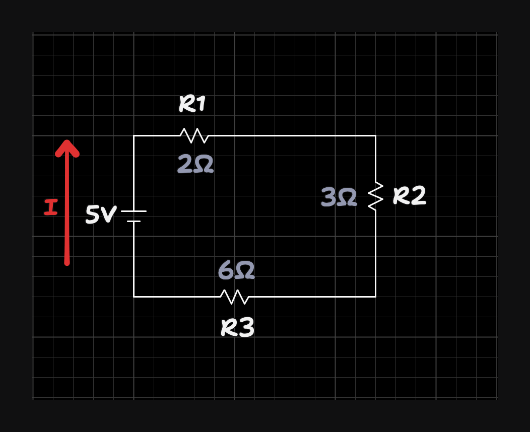
Component Values:

$V_1 = 5V, \quad R_1 = 2\Omega, \quad R_2 = 3\Omega, \quad R_3 = 6\Omega$

4.1 Kirchhoff's Laws Analysis

We'll start by analyzing the circuit using Kirchhoff's Laws, a method most are familiar with from class. This will serve as a foundation for understanding the connection to the Nodal Analysis method presented later.

I. Equivalent Resistance:
In a series circuit, the equivalent resistance is the sum of all resistances:

$R_{eq} = R_1 + R_2 + R_3 = 2Ω + 3Ω + 6Ω = 11Ω$

II. Total Current:
Using Ohm's Law ( $V = IR$ ), we can find the total current flowing through the circuit:

$I = \frac{V_1}{R_{eq}} = \frac{5V}{11Ω} \approx 0.45A$

III. Voltage Drops:
The voltage drop across each resistor is then calculated using Ohm's Law:

$V_{R1} = I \cdot R_1 = 0.45A \cdot 2Ω = 0.9V$

$V_{R2} = I \cdot R_2 = 0.45A \cdot 3Ω = 1.36V$

$V_{R3} = I \cdot R_3 = 0.45A \cdot 6Ω = 2.73V$

IV. Verification:
Kirchhoff's Voltage Law (KVL) states that the sum of voltage drops around a closed loop is zero.

$\begin{aligned} V_{R1} + V_{R2} + V_{R3} &= 5V \\ I \cdot R_{1} + I \cdot R_{2} + I \cdot R_{3} &= 5V \\ \frac{5}{11} \cdot 2 + \frac{5}{11} \cdot 3 + \frac{5}{11} \cdot 6 &= 5V \\ \frac{5}{11} \cdot (2 + 3 + 6) &= 5V \\ \frac{5}{11} \cdot 11 &= 5V \\ 5V &= 5V \\ \end{aligned}$

$0.9V + 1.36V + 2.73V \approx 5V$

This confirms our calculations.

4.2 Nodal Analysis

Nodal analysis is a more general method for solving circuits, based on Kirchhoff's Current Law (KCL). While it's more complex than necessary for this simple series circuit, it demonstrates a technique applicable to a wider range of circuit topologies.

I. Node Identification:

We'll label the node between R1 and R2 as $V_A$ .
We'll label the node between R2 and R3 as $V_B$ .
The bottom wire is our reference node (ground), with a voltage of 0V.

II. KCL Equations:

For Node A:

The current entering node A is $\frac{5 - V_A}{2}$ (from the voltage source through R1).
The current leaving node A is $\frac{V_A - V_B}{3}$ (through R2 to node B).

Applying KCL (current in = current out):

$\frac{5 - V_A}{2} = \frac{V_A - V_B}{3}$

For Node B:

The current entering node B is $\frac{V_A - V_B}{3}$ (from node A through R2).
The current leaving node B is $\frac{V_B - 0}{6}$ (through R3 to ground).

$\frac{V_A - V_B}{3} = \frac{V_B}{6}$

III. Matrix Form:
We can rewrite these equations in matrix form:
$\begin{bmatrix} \frac{1}{2} + \frac{1}{3} & -\frac{1}{3} \\ -\frac{1}{3} & \frac{1}{3} + \frac{1}{6} \end{bmatrix} \begin{bmatrix} V_A \\ V_B \end{bmatrix} = \begin{bmatrix} \frac{5}{2} \\ 0 \end{bmatrix}$

Simplifying the matrix, we get:

$\begin{bmatrix} 0.833 & -0.333 \\ -0.333 & 0.5 \end{bmatrix} \begin{bmatrix} V_A \\ V_B \end{bmatrix} = \begin{bmatrix} 2.5 \\ 0 \end{bmatrix}$
Solving this matrix equation (using methods like Gaussian elimination or matrix inversion), we get:
$\begin{bmatrix} V_A \\ V_B \end{bmatrix} \approx \begin{bmatrix} 4.09 \\ 2.73 \end{bmatrix}$

Therefore, $V_A \approx 4.09V$ and $V_B \approx 2.73V$ .

IV. Voltage Drops:
Now we can calculate the voltage drops across each resistor:

$V_{R1} = 5 - V_A = 5 - 4.09 = 0.91V$

$V_{R2} = V_A - V_B = 4.09 - 2.73 = 1.36V$

$V_{R3} = V_B = 2.73V$

These results are consistent with those obtained using Kirchhoff's Laws.

4.3 Program Output

The solver outputs these results as displayed in the following table, derived from the voltage drop calculations above:

Component	Value	Calculated Voltage
R1	2Ω	0.91V
R2	3Ω	1.36V
R3	6Ω	2.73V

5. Misc

5.0 Memorable Difficulties

UI-Components: There didn't seem to be any UI component libraries online that could be used to create a circuit editor UI. I had to create my own UI components from scratch and design the SVG paths bit by bit, which was a challenge in itself...
Time Constraints: Looking back, my goal for this project was too ambitious. Maybe due to naive expectations on the difficulty and also myself, I wanted to create a fully functional circuit solver and simulator, and even a user interface to go along with it. Yet the disproportionately long development cycle and lack of existing resources made it difficult to complete even a fraction of the project within the allotted time. I feel like I might have to switch this into a research project because this really is too difficult. But I already put so much time into this, there are no words that can express my frustration...

5.1 Limitations

Component Library: The current component library is limited to basic resistors (maybe capacitors) and voltage/current sources. More complex components (e.g., transistors, op-amps) could be added in the future.
Numerical Accuracy: With my current plan, the accuracy of the simulation would depend on the time step size and the numerical integration method used. Smaller time steps and more advanced integration methods can improve accuracy but increase computational cost.
Non-Ideal Components: The current implementation assumes ideal components. Incorporating non-ideal behavior (e.g., resistor tolerances, capacitor leakage) would enhance the realism of the simulation.

5.2 Future Improvements

Expand Component Library: Add more complex components like diodes, transistors, and operational amplifiers.
Implement AC Analysis: Enable the solver to analyze circuits with sinusoidal inputs and determine frequency responses.
Improve Numerical Methods: Explore more advanced numerical integration techniques for greater accuracy and efficiency in simulations.
Non-Ideal Component Modeling: Incorporate models for non-ideal component behavior to enhance simulation realism.
Sub-circuit Support: Allow users to create, save, and reuse sub-circuits to simplify the design of larger circuits.
Advanced Visualization: Implement more sophisticated visualization techniques, such as color-coded voltage and current flow graphs / animations.
Export/Import Functionality: Allow users to save and load circuits from files or to formats like SVG or TikZ.

6. Research Findings

It didn't seem appropriate to include this earlier in the document. I want to keep it separate from the main report.

Method	Description	Time Complexity	Accuracy	Advantages	Disadvantages	Best Suited For
Kirchhoff's Laws	Direct application of KCL and KVL to form a system of equations.	$O(N^3)$ or $O(B^3)$ ( $N$ = nodes, $B$ = branches)	Exact (within numerical)	Simple for basic circuits, provides exact solutions.	Cubic complexity can become a bottleneck, less straightforward for non-linear components or transient analysis.	Small, linear circuits with relatively few components.
Modified Nodal Analysis (MNA)	Systematic method combining KCL, KVL, and branch equations into a matrix form.	$O(N^3)$ (can be less with sparse matrix techniques)	Exact (within numerical)	General, handles a wide range of elements, sparsity can improve efficiency.	Can still be cubic complexity, more complex to implement than basic Kirchhoff's.	Moderate to large circuits, including those with voltage sources and complex components.
Nodal Analysis	Simplified MNA focusing on node voltages.	$O(N^3)$ (can be less with sparse matrix techniques)	Exact (within numerical)	Easier to implement than MNA, especially for circuits without many voltage sources.	Less general than MNA, may be less efficient with many current sources or complex branch relationships.	Circuits where branch currents are easily expressed in terms of node voltages.
Mesh Analysis	Another MNA specialization using mesh currents as unknowns, suitable for planar circuits.	$O(M^3)$ ( $M$ = meshes)	Exact (within numerical)	Can be simpler than MNA for planar circuits with many voltage sources.	Limited to planar circuits, not as general as MNA.	Planar circuits with numerous voltage sources.
Relaxation Methods	Iterative techniques (Gauss-Seidel, SOR) refining an initial guess until convergence.	Variable, depends on convergence rate	Approximate	Can be efficient for large, sparse systems and non-linear circuits.	Convergence not guaranteed, sensitive to initial guess, may require more iterations for complex circuits.	Large, sparse systems, circuits with non-linear components.
Charge Behavior Simulation (My Initial Approach)	Simulating the movement of individual charges over time.	$O(C \cdot F \cdot T)$ ( $C$ = charges, $F$ = per-charge complexity, $T$ = time steps)	Approximate	Handles non-linear components and transient behavior naturally, provides detailed insights.	Very computationally expensive, approximate solutions dependent on simulation parameters, requires detailed component models.	Circuits with complex device behavior, transient analysis where detailed charge movement is important.
Hybrid Methods (A Completely Made-up Approach..)	Combining various techniques (e.g., MNA formulation with mixed solvers and simplified models).	Highly variable, depends on the combination of methods	Varies	Should achieve a balance between accuracy and speed, handling a wide range of circuits and complexities.	Can be complex to implement, but should be possible.	General-purpose circuit simulation, aiming for efficiency and accuracy across different scenarios.

Note:

N: Number of nodes
B: Number of branches
M: Number of meshes
C: Number of charges simulated
F: Complexity of calculations per charge per time step
T: Number of time steps

A large part of this project was about trying to strike a balance between accuracy and speed, and how to handle a wide range of circuits and complexities. This table provides an overview of the characteristics, advantages, disadvantages, and suitability of each method. The best method for a specific circuit problem will depend on the specific requirements and constraints of that problem. Determining those constraints is most likely the key to successful and efficient circuit simulation.

Now with this in mind, continuing from Part 4: (My analysis and execution might not be elegant, but these are all the methods I researched and considered)

4.4 Modified Nodal Analysis (MNA)

Description: A systematic and general method for solving circuits. It combines KCL, KVL, and branch constitutive equations (e.g., Ohm's Law) into a matrix form. Handles a wide variety of circuit elements, including voltage sources, current sources, and more complex components.

Walkthrough Example:

Using the same circuit as in the nodal analysis example:

alt text

Component Values:

$V_1 = 5V, \quad R_1 = 2\Omega, \quad R_2 = 3\Omega, \quad R_3 = 6\Omega$

1. Identify Nodes and Branches: We have nodes labeled $V_A$ , $V_B$ , and a reference node (ground). We have branches containing R1, R2, R3, and V1.

2. Assign Node Voltages: Assign voltages $V_A$ and $V_B$ to nodes A and B, respectively.

3. Apply KCL at Nodes:

Node A: $\frac{V_1 - V_A}{R_1} + \frac{V_B - V_A}{R_2} = 0$
Node B: $\frac{V_A - V_B}{R_2} - \frac{V_B}{R_3} = 0$

4. Include Equations for Voltage Sources: $V_1 = 5$

5. Formulate the MNA Matrix: We can rewrite the equations in matrix form, incorporating the voltage source V1 directly into our equations. Since V1 is connected between the source and node $V_A$ , we can express $V_A$ in terms of $V_1$ :

$V_A = V_1$

Substituting $V_1 = 5$ into the KCL equations and simplifying, we get:

Node A: $\frac{5 - V_A}{2} + \frac{V_B - V_A}{3} = 0$

$1.5 \cdot 5 - 1.5 V_A + V_B - V_A = 0 => 2.5 V_A - V_B = 7.5$

Node B: $\frac{V_A - V_B}{3} - \frac{V_B}{6} = 0$

$2(V_A - V_B) - V_B = 0 => 2 V_A - 3 V_B = 0$

This system simplifies to two equations:
$\begin{cases} 2.5 V_A - V_B = 7.5 \\ 2 V_A - 3 V_B = 0 \end{cases}$
We can represent this in matrix form as:
$\begin{bmatrix} 2.5 & -1 \\ 2 & -3 \end{bmatrix} \begin{bmatrix} V_A \\ V_B \end{bmatrix} = \begin{bmatrix} 7.5 \\ 0 \end{bmatrix}$

Solve the Matrix Equation: Solving this system of equations (using Gaussian elimination, LU decomposition, or other methods), we get:
$\begin{bmatrix} V_A \\ V_B \end{bmatrix} = \begin{bmatrix} 4.09 \\ 2.73 \end{bmatrix}$

Thus, $V_A = 4.09V$ and $V_B = 2.73V$ , which matches the previous results from nodal analysis.

Time Complexity: $O(N^3)$ , where N is the number of nodes and additional variables introduced by voltage sources and other elements. However, the use of sparse matrix techniques can significantly reduce this complexity for large circuits.

Accuracy: Exact (within numerical precision limits).

Advantages:

General and versatile, capable of handling a wide range of circuit elements, including voltage sources, current sources, and more complex components.
Systematic approach, making it suitable for implementation in software.
Sparsity of the MNA matrix can be exploited to improve efficiency for large circuits.

Disadvantages:

Can still have cubic complexity, although sparse matrix techniques mitigate this.
More complex to implement than basic Kirchhoff's Laws or nodal analysis.

Best Suited For: Moderate to large circuits, including those with voltage sources, current sources, and complex components.

4.5 Nodal Analysis

Description: Nodal Analysis is a specialization of MNA that focuses on node voltages as the primary unknowns. It is particularly well-suited for circuits where branch currents can be easily expressed in terms of node voltages (e.g., using Ohm's Law).

Execution:

We've already covered a detailed nodal analysis walkthrough in Section 4 of the main report. Here's a summary:

1. Choose a Reference Node:
Usually ground.

2. Assign Voltages to Other Nodes:
These are the unknowns

3. Apply KCL at Each Non-Reference Node:
Express currents in terms of node voltages and resistances

4. Solve the System of Equations:
The resulting system of equations is solved to find the node voltages.

Time Complexity: $O(N^3)$ , where N is the number of nodes. Sparse matrix techniques may improve this.

Accuracy: Exact (within numerical precision).

Advantages:

Simpler to implement than full MNA, especially for circuits without many voltage sources.
Efficient for circuits where branch currents are easily expressed in terms of node voltages.

Disadvantages:

Less general than MNA. Can be less efficient if there are many current sources or complex branch relationships.

Best Suited For: Circuits where branch currents are easily expressed in terms of node voltages. (If you already have MNA, there is no reason to look at this method for obvious reasons)

4.6 Mesh Analysis

Description: Mesh Analysis is another specialization of MNA that uses mesh currents (currents circulating in the loops of a planar circuit) as the primary unknowns. It's particularly useful for planar circuits with many voltage sources. As you can probably tell by now, each method has its own advantages and disadvantages. This is actually the most interesting part of the report !

Walkthrough Example:

Consider a simple planar circuit with two meshes:

Identify Meshes: Assign mesh currents (e.g., I1, I2) to each independent loop
Apply KVL around each mesh: Express voltage drops in terms of mesh currents and resistances
Solve the System of Equations: Solve for the mesh currents. Branch currents can then be calculated from the mesh currents

Time Complexity: $O(M^3)$ , where M is the number of meshes.

Accuracy: Exact (within numerical precision).

Advantages:

Can be simpler than nodal analysis for planar circuits with many voltage sources.

Disadvantages:

Limited to planar circuits.
Not as general as MNA.

Best Suited For: Planar circuits with numerous voltage sources.

4.7 Relaxation Methods (Iterative)

Description: Relaxation methods, such as Gauss-Seidel and Successive Over-Relaxation (SOR), are iterative techniques that start with an initial guess for the solution and refine it until convergence is achieved.

Walkthrough Example (Gauss-Seidel):

Formulate Equations: Express the equations in a form suitable for iterative solution (e.g., $x_i = f(x_1, x_2, ..., x_n)$ ).
Initial Guess: Provide an initial guess for all unknowns.
Iterate: Update each unknown using the most recently calculated values for the other unknowns.
Convergence Check: Check if the solution has converged (e.g., if the change in values between iterations is below a threshold). Repeat steps 3 and 4 until convergence (may take forever).

Time Complexity: Variable, depends on the convergence rate.

Accuracy: Approximate. The accuracy depends on the convergence criteria.

Advantages:

Can be efficient for large, sparse systems.
Can handle non-linear circuits.

Disadvantages:

Convergence is not guaranteed. This is the main caveat.
Sensitive to the initial guess.
May require many iterations for complex circuits.

Best Suited For: Large, sparse systems, circuits with non-linear components.

4.8 Charge Behavior Simulation (My Initial Approach Lol 🤡)

Description: This approach involves simulating the movement of individual charges within the circuit based on electric fields and component behavior.

Walkthrough:

Model Components: Define how each component affects charge movement (e.g., resistors impede flow, capacitors store charge).
Initialize Charges: Distribute various charges as "probes" within the circuit, closing a path once a charge traverses it.
Time Steps: In discrete time steps, update the position and velocity of each charge based on the electric fields and component interactions.
Calculate Currents and Voltages: Derive macroscopic quantities (currents, voltages) from the movement of charges.

Time Complexity: $O(C \cdot F \cdot T)$ , where C is the number of charges, F is the complexity of calculations per charge per time step, and T is the number of time steps.

Accuracy: Approximate, depends on the simulation parameters (time step, number of charges).

Advantages:

Handles non-linear components and transient behavior naturally.
Provides detailed insights into charge movement.

Disadvantages:

Very computationally expensive.
Approximate solutions dependent on simulation parameters.
Requires detailed component models.

Best Suited For: Circuits with complex device behavior, transient analysis where detailed charge movement is important. Not practical for large circuits.

4.9 Hybrid Methods (A Completely Made-up Approach.. 🤡)

Description: Hybrid methods would combine different techniques to leverage their strengths. For example, MNA could be used to formulate the circuit equations, but then a relaxation method could be used to solve the resulting system of equations. Simplified models for some components could be used to reduce complexity. There are many combinations possible, which makes this very very interesting.

Walkthrough: Highly variable depending on the specific hybrid approach.

Time Complexity: Highly variable.

Accuracy: Varies.

Advantages:

Has the most potential to achieve a balance between accuracy and speed among all methods.
Would be able to handle a wide range of circuits and complexities.

Disadvantages:

Can be complex to implement, but very feasible.

Best Suited For: General-purpose circuit simulation, aiming for efficiency and accuracy across different scenarios. Requires careful design and selection of appropriate methods.

This probably already exists somewhere in the wild, considering there are 8 billion people on the planet. But I think finding the right combination of methods is a timeless challenge in the realm of circuit simulation. And that's what this project is all about!

7. Conclusion

This project researched and developed circuit solver and simulator methods that goes beyond the concepts covered in class by implementing advanced analysis techniques and dynamic simulation capabilities. The project demonstrates a strong understanding of electrical circuit principles, numerical methods, and software development through the time complexity analysis of various methods. The resulting software provides a valuable tool for learning, experimenting with, and analyzing electrical circuits. The project also highlights the importance of connecting theoretical knowledge to real-world applications and provides a foundation for further exploration into the field of circuit simulation and design.

8. Time Log (`-` for ongoing)

Task	Time Spent (hours)
Research and Planning	10
UI Design and Implementation	16.1
Circuit Representation and Data Structures	19.7
Nodal Analysis Solver Implementation	8.2
Simulation Engine Implementation	-
Testing and Debugging	NO
Report Writing	8.5
Total	62.5

9. References

Stack Exchange (Initial Research):

More Technical References (In-Depth):

Grounding References (Precedes all technical aspects):

+all references from Section 6 of report

My research journey began with exploratory browsing on Stack Exchange to gain an initial understanding of circuit solving and simulation approaches. This groundwork laid the foundation for my initial plan. Subsequently, I delved into more technical literature to explore specific methods in greater depth.

During this phase, I frequently encountered concepts that were impossible for me to grasp independently. I tried using ChatGPT as a tool to aid in understanding these complex topics, but you cannot rely on a probabilistic model for technical accuracy.

So I named the third category "grounding". These resources provided a more tangible foundation in the basic principles, which was the only way to achieve a true understanding of the more advanced material.

Interestingly, I only discovered that first Stack Exchange post towards the end of my snooping around and binging. It was like a missing piece, connecting the various concepts explored and revealing the broader context of circuit analysis methods.

The entire process felt like navigating a rabbit hole. Each resource led to new questions and deeper investigations. Based on my current understanding, I hypothesize that the ultimate solution for optimal circuit analysis might lie in a machine learning model.

Such a model could potentially integrate the collective knowledge from existing research, intelligently selecting and combining the most efficient methods for any given circuit. This is feasible because decades of research have extensively explored and refined various circuit analysis techniques. The strengths, weaknesses, and ideal use cases for each method are now well-understood.

However, these individual pieces of knowledge often exist in isolation. A machine learning model could bridge this gap by combining the collective knowledge from existing research, effectively integrating the strengths of each approach to achieve unprecedented efficiency and accuracy in circuit analysis.

Circuit Solver and Simulator: A Deep Dive into Electrical Networks 🙂✨

1. Introduction

2. Theoretical Background

2.1 Nodal Analysis

2.2 Circuit Simulation:

3. Implementation

3.1 Circuit Representation

3.1.1 UI to Graph Conversion (Challenges)

3.2 Nodal Analysis Solver

3.3 Circuit Simulation Engine

3.4 User Interface:

Editor:

4. Quantitative Analysis and Results

4.1 Kirchhoff's Laws Analysis

4.2 Nodal Analysis

4.3 Program Output

5. Misc

5.0 Memorable Difficulties

5.1 Limitations

5.2 Future Improvements

6. Research Findings

4.4 Modified Nodal Analysis (MNA)

4.5 Nodal Analysis

4.6 Mesh Analysis

4.7 Relaxation Methods (Iterative)

4.8 Charge Behavior Simulation (My Initial Approach Lol 🤡)

4.9 Hybrid Methods (A Completely Made-up Approach.. 🤡)

7. Conclusion

8. Time Log (- for ongoing)

9. References

8. Time Log (`-` for ongoing)